This post is meant as a companion to our EMNLP 2016 paper “Building an Evaluation Scale using Item Response Theory”. It’s quite a bit overdue, but hopefully this post will be useful to those who haven’t seen IRT before.
Introduction
Let’s start by thinking about the typical supervised machine learning setup. There is some training data, a held-out test set, and a machine learning model. The goal is to use the training data to learn a model that performs well on the test set. “Performs well” is usually measured by some aggregate statistic such as accuracy, precision/recall, etc. These aggregate statistics assume that each test set example is as important in determining model performance as every other test set example. But what if that isn’t the case? What if certain examples are so easy that labelling them incorrectly is disastrous? Or on the other hand, what if certain examples are so hard that no model labels them correctly (except your new deep deep deep network)?
Characteristics such as difficulty are often used to assess humans in psychometrics, specifically a method known as Item Response Theory (IRT). The high-level idea with IRT is that if you have enough test-takers providing answers to questions on a test (“items,” hence the Item in IRT), you can learn latent parameters of the items as well as estimate a latent ability trait of the test-takers themselves. IRT is popular in standardized tests such as the SAT and the GMAT. It’s used to assess the test-takers but also to select appropriate items for the tests themselves (if a test question is too easy, there’s no need to include it). What we wanted to do was take the IRT methodology and apply it to machine learning models, specifically models trained to do the natural language processing (NLP) natural language inference (NLI) task.
IRT
The key driver behind IRT is what’s known as the Item Characteristic Curve (ICC). Each item has an associated ICC, which can take certain forms depending on the IRT model that you’re looking at. A popular model (and the one we used in our paper) is the 3 Parameter Logistic (3PL) model:
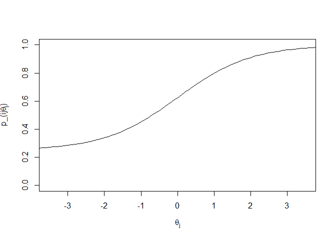
\[p\_{ij}(\theta_j) = c_i + \frac{1 - c_i}{1 + e^{-a_i(\theta_j - b_i)}}\]Here, θj is the latent ability parameter of test-taker j, and ai, bi, and ci are item i’s discriminatory, difficulty, and guessing parameters, respectively. A typical IRT curve will look something like this:

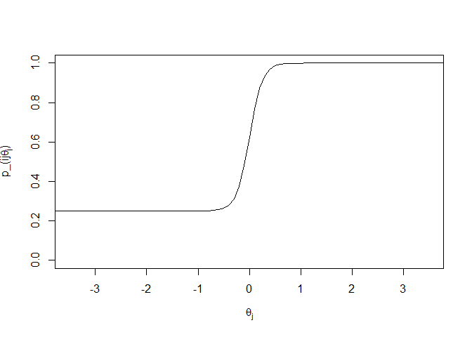
Our x-axis is θj, the latent ability parameter. The y-axis is pi**j(θj), the probability that an individual with a certain ability level will answer this item correctly. The curve is monotonically increasing, which makes sense. As the ability of an individual increases, we expect that the probability of that individual answering correctly will also increase. ai, the discriminatory parameter, represents the slope of the curve at its steepest point. ai should be steep enough that in a relatively short range, there is a sizeable jump in pi**j(θj), but shouldn’t be so steep that the range is tiny. An item with too steep of a slope is only useful in a very small ability range:

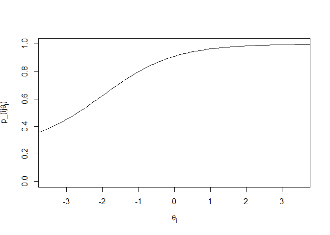
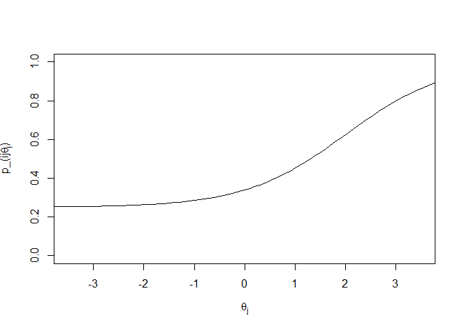
bi, the difficulty parameter, represents the halfway point between the minimum and maximum values of pi**j(θj). For a 3PL model, the minimum is ci and the maximum is 1. Since θ is a unit Gaussian (θj ∼ N(0, 1)), we want the value of bi to fall somewhere between −3 and 3 in most cases, since that covers 99.7% of people. The next two plots show “easy” and “hard” items where the difficulty parameters are −2 and 2, respectively:


ci is referred to as the guessing parameter. As you can see from the plots above, the lower asymptotes of the curves are not 0. In a three parameter model, there is an assumption that even at low levels of θ, there is some non-zero probability that an individual will answer a question correctly (with for example a lucky guess). That is modeled by ci.
IRT for NLP
So how can we use IRT to help us in NLP? It’s often the case that when you train and test your brand new machine learning model on an NLP dataset, the metric of interest is test set accuracy. If your model has a higher accuracy than the current state of the art in the literature, then your model becomes the new benchmark against which other models are evaluated. However, there is usually something missing in these evaluations: the question of the specific test set examples that were answered correctly. If your fancy new model has a high accuracy because it labeled a random sequence of examples correctly, that indicates very different performance than some other model that labeled items correctly according to their difficulty (i.e. labeled all easy examples correctly up to some difficulty threshold, then labeled all subsequent examples incorrectly). Having some notion of difficulty is important to distinguish between these two cases, which is where IRT comes in!
We decided to test this out on the Stanford Natural Language Inference (SNLI) dataset. Natural language inference (NLI) is a popular task in NLP, where the goal is to determine if some sentence (premise) entails some other sentence (hypothesis). If the premise is true, does that mean that the hypothesis must be true (entailment), cannot be true (contradiction), or could be either (neutral)? You can imagine that there might be some ambiguity about certain examples having certain labels. So this seems like a perfect place to apply IRT to see if we can learn anything about the data and the high-performing models trained on the dataset.
Data Collection
In order to fit these IRT models, you need a lot of data. Specifically, you need a lot of answers to the same set of questions. If you ask a lot of people to take the same test, then grade each of their answers, the graded responses for each person is that person’s response pattern. With a set of response patterns you can fit an IRT model to learn the latent parameters of the items as well as the latent θ for each of the test-takers.
This goes against what is typically done when you are gathering data for machine learning models. Usually, you will collect between one and five labels for each example in your data set, and use a majority vote to determine the gold standard. Here, we used the crowdsourcing platform Amazon Mechanical Turk to gather 1000 labels for each example from our SNLI subset. So instead of asking a lot of Turkers for a few labels to a lot of examples, we asked them for a lot of labels for a small number of examples. Each Turker provided a label for each example, so we were able to grade the Turker responses to generate response patterns.
IRT Analysis
Fitting an IRT model is a cyclical process. At a high level, you fit your model, using your software package of choice (for R, the mirt package is a good one). Then you check how well each item fits in with the learned model. Are there items where the discriminatory parameter is too large? Items like these aren’t useful outside of a very specific range so they can be removed. Items where the parameter is too small are also removed, because they are not able to discriminate at all. Are there items that violate the local independence assumption? These are also removed. Typically the items are removed one at a time, the model is re-fit, and the set of items is checked again.
Results
There are a number of results in the paper, but to boil it down into a single takeaway: specific data points are important! If you are testing your model on an easy dataset, then high accuracy scores aren’t all that impressive, because everyone has a high accuracy. On the other hand, if you test on a difficult dataset, then lower accuracy scores may be indicative of higher latent θ, since the score is with respect to some population of test-takers.
Conclusion
Hopefully this was a useful introduction to IRT. I encourage you to check out the paper for much more detail. And feel free to email me if you have any questions or comments. The next post will discuss our EMNLP 2018 paper: Understanding Deep Learning Performance through an Examination of Test Set Difficulty: A Psychometric Case Study.
